Assignment 7: Motion planning

One of the fundamental problems in robotics is motion planning: given a robot R and an environment (or physical space), a start and end position p_start and p_end, find a path so that the robot can move from start to end, without collisisons.

Sometimes, depending on the problem, we might want the shortest path from p_start to p_end, other times just a path (not necessarily the shortest) may be sufficient.

The general motion planning problem is quite difficult. We'll make some simplifying assumptions:

We'll look at the 2-dimensional motion planning problem. That is, the robot is moving in a 2D environment. Most generally, the robot will be some sort of 2D-polygon (convex or not), and we'll assume it does not have joints (not an articulated robot), and the environment consists of a set of 2D polygons that represent the obstacles.
We'll assume that the environment is static (the obstacles are fixed).
The environment is known, ie the robot knows the list of obstacles with their vertices and edges. That is, the robot does not rely on sensors to learn the environment, instead the environments is given.

Notation: we'll assume that the obstacles consist of n edges. So for us O(n) represents the complexiy of the obstacles (vertices plus edges). We assume that the robot is moving in a large bounding box B that contains all polygons.

The general idea

The general idea of motion planning is to start by computing a decomposition of the free space (the space where the robot can move) into cells, and construct a road map of the free space to guide the motion between neighboring cells. This road map is essentially a graph through free space. Ideally we want to build the roadmap so that so that we are able to say that:

any path in the road map corresponds to a collision-free path in the free space.
any path in the free-space corresponds to a path in the road map.

Once the roadmap is computed, essentially we have reduced the motion planning problem to a path problem in a graph.

A point robot moving among polygonal obstacles in 2D:

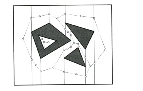
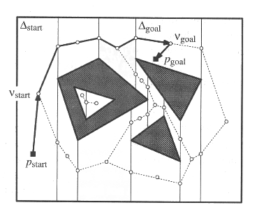
The simplest example is that of a point robot moving among polygonal obstacles. The free space can be decomposed as follows: from each vertex, shoot a vertical ray above and below, until it intersects with an edge (or the bounding box B). This is called a trapezoidal decomposition, and we have seen something very similar when we talked about polygon triangulation (here we have a set of polygons, not just one). This trapezoidal decomposition can be computed using standard techniques. Each trapezoid corresponds to a region of the free space. To guide movement between adjacent trapezoids, we can construct a road map as follows: we place one node in the center of each trapezoid, and we place one node in the middle of each vertical edge. There is an arc between two nodes if and only iff one node is in the center of a trapezoid and the other node is on the boundary of that same trapezoid. The figure below illustrates this (from 4M book). A path from start to end can be found via BFS in the road map. It can be shown that the road map has linear complexity O(n), which is good. But, paths obtained with this approach are not necessarily shortest.

A different type of road map that can be used for finding shortest paths is the visibility graph: this is a graph whose vertices are the vertices of the obstacles, and its edges (u,v) are all the pair of vertices that can "see" each other, that is, segment uv does not intersect the interior of any obstacle. Below is a screenshot from http://www.cs.cmu.edu/afs/cs.cmu.edu/academic/class/16311/www/s06/lecture/lec8.html.

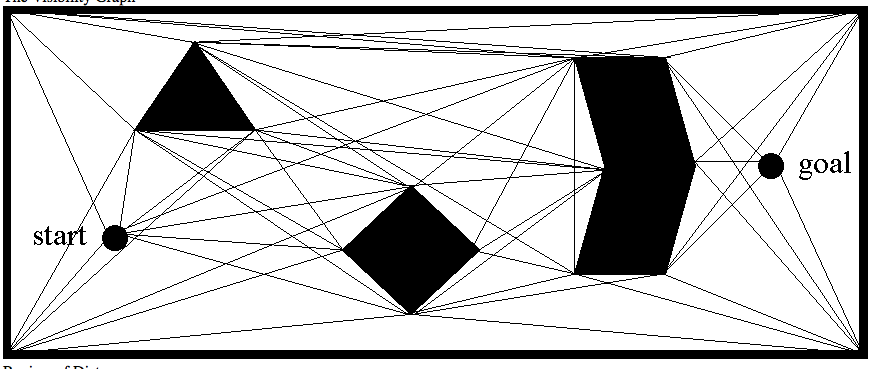
In class we'll talk about this in more details, and show that shortest paths in 2D have the very nice and convenient property that they are srtaight lines, and they have to go through the polygonal vertices. This basically means that any shortest path will be contained in the VG. Once the visibility graph (VG) is computed, the shortest paths from start to end can be computed for e.g. using Dijkstra's algorithm. The problem with this approach is that the VG may have quadratic complexity in the worst case, and any approach that computes the whole VG is doomed to quadratic complexity.

This assignment part I: a point robot moving among polygonal obstacles

Assume a point robot moving in 2D. Generate a scene consisting of multiple polygonal obstacles and a start and end position. Have a pre-set scene, but also allow the user to enter the obstacles by clicking the mouse.
Compute and render the visibility graph.
Run Dijkstra's algorithm on the VG and render the resulting path in a different color.

Towards a more general case

Now that we got the basics working, we can move on to more realistic scenarios. We'll consider that the robot is a convex polygon. For simplicity, we'll assume it's a rectangle.

In this scenario we need to start taking about the configuration space, in addition to the physical space: the physical space is the space where the robot is moving. The configuration space is the parametric space where the robot is moving; put differently, it's the set of all positions for the robot.

For example: when the robot is a rectangle and can only translate, this means that its position at any time is fully specified by two coordinates: (x,y). Think of these as the coordinates of its center. Each position of the robot would correspond to a point in a 2-dimensional parametric space (the configuration space). We can view the physical movement of the robot as a move in the parametric or configuration space; in this case the parametric space is also a 2D space.
If the robot would be able to rotate, then its position would be specified by 3 parameters: (x,y, theta). Each position of the robot would correspond to a point in this 3-dimensional parametric space. The robot would be moving physically in a 2D space, and parametrically in a 3D space.
The parametric space corresponds to the degrees of freedom (dof) of the robot, and you can imagine its gets pretty complicated with articulated arms and such.

We view the motion of the robot as a path in the physical 2D space, and associate with it a path in its parametric space. Remember that a path in physical space has to be collision-free. We have to extend the concept of obstacles. Obstacles exist in physical space, and we need to generalize them to parametric space. Consider a robot R and a physical obstacle O; the parametric obstacle PO corresponding to the real obstacle O can be defined as follows: a point (x,y) is part of PO if placing the robot R at position (x,y) would cause a collision with obstacle O.

The free configuration space represents all points in parametric space that are not part of parametric obstacles.

The basic steps of generic motion planinng are as follows:

For each obstacle O, compute its coresponding parametric obstacle (Minkowski sums of the robot and the obstacke)
Compute the union of all parametric obstacles
Compute their complement (this represents the free configuration space).
Compute a roadmap for the free configuration space, and use it to find paths.

This way, motion planning of a general robot is framed as motion planning of a point robot moving in parametric space. Efficient solutions are known for all intermediate steps for a bunch of simple cases (essentially for convex robots movving among convex polygons, and only translations are allowed).

Heuristics: In many practical situations, computing the free configuration space and a complete roadmap is too costly or is not possible. However, this idea of framing motion planning as a search in parametric space is nice and convenient, because it allows for artificlal intelligence heuristics. A common idea in many approaches is to discretize free space and approximate it with a grid. This is what you'll implement for the second part of this assignment.

Assignment part 2: a rectangular robot translating among polygonal obstacles

In this part, your robot is a rectangle. Let's say it has pre-set size and start position. Find a collision-free path of the robot from start to end, by performing a search in the 2d-dimensional paramatric search that correspnds to the position of the center of the robot. Below is a generic search procedure:

a state is a position (x,y) of the robot 
Q is a queue (priority queue) of  states 
initially Q contains the start position

while  goal not found
     remove state s from Q
     find all successors of state s (all states where we can move from s)
     for each such successor s':
              if s' is the final goal state, then we are done;
              otherwise check that we have not been there (at s'); if we have, skip to next successor
             check whether placing the robot at s' would intersect any obstacle; if not,   put s' on the queue

To guide the search towards the goal, score each state with a cost function that adds two components: the euclidian distance of that state from the goal state, and the euclidian distance form the start state.

Approximate the parametric space with a grid. What this entails, for your algorithm, is how you generate the successor states: a state (x,y) can move only to its 4 neighbors on the grid: (x, y+1), (x, y-1), (x-1, y), (x+1, y). You could also allow diagonal moves, that might speed up teh search. Assume the resolution of the space is the resolution of the window (500 by 500?).

Testing for intersections: your basic interscetion function will be to test whether the robot, when placed at (x,y), would stay completely in free space. One way to do this is to check, for each of its 4 edges, whether it intersects any obstacle edge (you'll need to think of something to detect when robot is completely inside a polygon). Another idea is to pre-process the scene in an occupancy grid: this is a grid that stores, for each pixel in your discretized parrametric space, whether that pixel is free, or occupied (falls inside an obstacle). If you have an occupancy grid, then you can use it to determine whether a state is intersection free, by essentially checking every pixel that the robot occupies to see if it is free or not.

Keeping track of the path: During the search, whenever a state discovers another state, set parent pointers appropriately. At the end, you'll be able to start from the goal and move through the parent pointers and find the path. The goal of the program woudl be to find and render this path.

Part III (for those who want a challenge, and fame): extending to rectangular robots that can translate and rotate among polygonal obstacles.

This sounds tricky, but if you implemented part II in a generic way, it comes for free. Here the parametric space is 3 dimensional. It comes down to writing a different function to generate next state; and writig a different function that tests whether a rectangle at (position (x,y) and rotated by alpha stays completely in free-space.

How to turn in: If you used the svn folder provided, there is no need to email me the files, I will access them in your svn folder. If you did not use the svn folder provided, you should.

Enjoy!