Terrains are represented by sampling points on the terrain and recording the geographical coordinates {x, y} of the point and the coresponding elevation {z} of the terrain at that point. Thus a terrain is represented as a cloud of points {x, y, z} stored in a file.
The most common terrain data available comes in form of a grid: this means that the points {x, y} are sampled uniformly with a grid. Grid elevation data is refered to as a digital elevation model or DEM, in short. In a grid terrain the individual coordinates {x, y} of the points need not be specified. It is sufficient if we know the coordinates of the upper-left corner of the grid and the spacing between sample points. If these are specified, the geographical coordinates of the grid points are implicit.
A grid terrain consists of a header, and a set of points {z} that represent the elevation of the terrain sampled with a uniform grid. Here is a grid file, set1.asc, that represents a basin in the Sierra Nevada range in the south-west. Open it and take a good look at it.
The format of a grid file is standard. The first 6 lines in the file represent the header of the terrain; it stores the number of rows in the grid, the number of columns, the geographical coordinates of the lower left corner, the spacing in the grid (assumed to be the same both horizontally and vertically), and a nodata value (this is the value that is used for points where the elevation could not be measured).
ncols         391
nrows         472
xllcorner     271845
yllcorner     3875415
cellsize      30
NODATA_value  -9999
Following the header there are nrows lines, each line containing ncols values, for a total of nrows * ncols values. These values represent the elevations sampled from the terrain. Thus, a grid terrain is basically a 2D-array of elevation values. You can assume that the elevations are integers (though you can also use floats or doubles if you want). The dimensions of the grid can be found out from the header. The other information stored in the header (xllcorner, yllcorner, cellsize, NODATA_value) you will happily ignore for this lab since we won't care about geographical coordinates---- but you have to read them anyways in order to get to the point in the file where you can start reading the elevations.
Reading a grid: The constructor
Grid (String fileName)should take a file name as parameter. It will open the file, read the header, create an elevation grid and load it with the values from the file. One thing you will need to figure out is how to work with files in Java.
File f = new File(fileName);
Scanner sc = null;
try {
     sc = new Scanner(f);
    } catch (FileNotFoundException e) {
     System.err.println("File not found!");
     System.exit(0);
    }

//here is how you would read a file of integers
while (sc.hasNextInt()) {
    int nextOne = sc.nextInt();

}
In a nutshell, the code creates a new File, then opens the file up with
the Scanner class. Opening a scanner from a file must be checked for
an exception to make sure everything went ok. Once it has been opened,
then the Scanner can basically act as an interator.
Here are some test grids. Some of them (europe.asc) are large, so better not open them in a browser. Your Grid class will not be able to handle large files (try it), but it should handle the rest of them just fine. While testing, I would try getting the small ones to work before I try any of the larger ones.
If you want to play with more data, you can download your own DEMs at USGS geodata site. One of the test DEMs I included, europe.asc, comes from this site under GTOPO30 project, which contains Global 30 Arc-Second Elevation Data Set global DEM with a horizontal grid spacing of 30 arc seconds (approximately 1 kilometer). These files come in a different format, so if you want to use one of them, let me know and I will convert it for you.
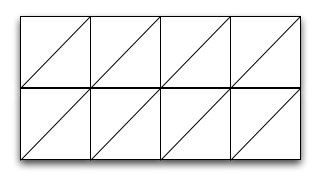
Rendering a grid: Class Grid should provide a function to render the grid in a window. To render a grid you will go through all the points (i,j) in the grid drawing lines between neighboring points so that overall the lines you draw form a triangulation as below:
You will use the position (i,j) of the point in the grid to determine the position (i', j') of the point in the window. You will use the elevation of point (i,j) to determine the color with which you draw the point.
The first thing you will need to figure out is how to convert from grid coordinates to window coordinates. You will need to scale the terrain to the window. Assume a square window, for simplicity. When displayed, the longest side of a terrain should match the window dimension. Note that we ignore true geographical coordinates, and we use (row, column) of the point--- we don't care about the true geographical location anyways, at least, not for this lab.
One way to do this is by computing two stretch factors, one horizontal and one vertical: stretch_horiz and stretch_vert.
i' = i * stretch_horiz;
j'= j * stretch_vert;
The stretch factors can be computed knowing the size of the window, and the dimensions of the grid. You may need to change the lines above to account for centering, if you need to.
Colors: On a real map elevations are coded using colors: high elevations are brown, low elevations are green. You will use the elevation of the terrain to choose the color with which you draw each line.
First, some background on colors. In Java the color is specified as a triplet (r, g, b), where r, g, b are values in the range [0.0, 1.0] specifying the red, green and blue intensity in the color, respectively. 0.0 represents the darkest, and 1.0 the lightest. WHITE corresponds to (1.0, 1.0, 1.0) and BLACK corresponds to (0.0, 0.0, 0.0).
Remember that on a graphics object you can change the color using
Color c = new Color (r, g, b);
g.setColor(c);
In order to make the color reflect the elevation, you will have to come up with a formula to set r,g,b as function of the elevation; you will need to do this every time you call drawLine, to set the color of the line as a function of the elevation of that line. Assume that the elevation of the line is the average of the elevation of its points.
To come up with a logic for setting r, g, b, remember that r, g, b must be values in [0.0, 1.0], with 0.0 corresponding to highest elevation, and 1.0 to lowest elevation.
The easiest way would be to set all of them to the same value. Equal values for r,g and b give a gray color, so it will result in a gray-scale image.
r = g = b = ...
c = new Color(r, g, b);
g.setColor(c)
| 
|
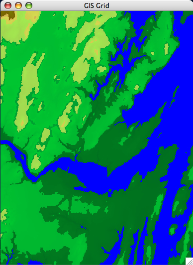
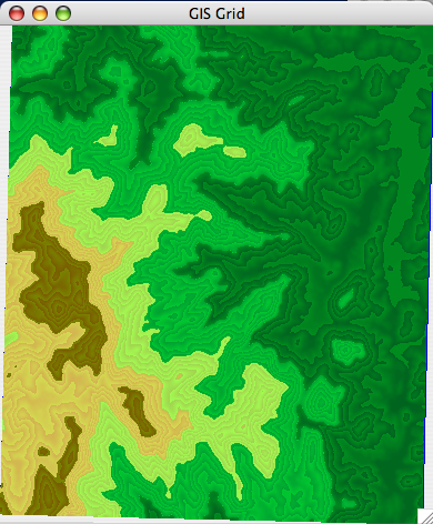
| [Brunswick DEM] | [set1 DEM] |
As usual, encapsulate, use small functions, write nice code, write code incrementally and debug it before you move to the next step.
Have fun!