Elevation data has traditionally been obtained by interpolating cartographic maps; elevation data can also be estimated based on radar images: Synthetic Aperture Radars (SAR) produce high resolution images of the Earth's surface providing useful information about the physical characteristics of the ground and of the vegetation canopy, such as surface roughness, soil moisture, tree height and bio-mass estimates. By combining two or more SAR images of the same area it is possible to generate elevation maps and surface change maps with unprecedented precision and resolution. This technique is called SAR interferometry. More recently elevation data is available (directly) from technologies like LIDAR.
In this lab you will develop an application to read terrain elevation data from a file, render it, and compute the flow of water on the terrain. These are basic functions in a Geographic Information System (GIS).
Terrains are represented by sampling points on the terrain and recording the geographical coordinates {x, y} of the point and the coresponding elevation {z} of the terrain at that point. Thus a terrain is represented as a cloud of points {x, y, z} stored in a file.
The most common terrain data available comes in form of a grid: this means that the points {x, y} are sampled uniformly with a grid. Grid elevation data is refered to as a digital elevation model or DEM, in short. In a grid terrain the individual coordinates {x, y} of the points need not be specified. It is sufficient if we know the coordinates of the upper-left corner of the grid and the spacing between sample points. If these are specified, the geographical coordinates of the grid points are implicit.
A grid terrain consists of a header, and a set of points {z} that represent the elevation of the terrain sampled with a uniform grid. Here is a grid file, set1.asc, that represents a basin in the Sierra Nevada range in the south-west. Take a good look at it.
The format of a terrain grid file is standard. The first 6 lines in the file represent the header of the terrain; it stores the number of rows in the grid, the number of columns, the geographical coordinates of the lower left corner, the spacing in the grid (assumed to be the same both horizontally and vertically), and a nodata value (this is the value that is used for points where the elevation could not be measured).
ncols         391
nrows         472
xllcorner     271845
yllcorner     3875415
cellsize      30
NODATA_value  -9999
Following the header there are nrows lines, each line containing ncols values, for a total of nrows * ncols values. These values represent the elevations sampled from the terrain. Thus, a grid terrain is basically a 2D-array of elevation values. You can assume that the elevations are integers (though you can also use floats or doubles if you want). The dimensions of the grid can be found out from the header. The other information stored in the header (xllcorner, yllcorner, cellsize, NODATA_value) you will happily ignore for this lab since we won't care about geographical coordinates---- but you have to read them anyways in order to get to the point in the file where you can start reading the elevations.
The constructor: Reading a grid from a file
Grid (String fileName)should take a file name as parameter. It will open the file, read the header, create the array to hold the elevation values, and load it with the values from the file. One thing you will need to figure out is how to work with files in Java. Below is a piece of code that opens a file, creates a scanner on it, and reads integers (while any).
Files in Java
File f = new File(fileName);
Scanner sc = null;
try {
     sc = new Scanner(f);
    } catch (FileNotFoundException e) {
     System.err.println("File not found!");
     System.exit(0);
    }

//here is how you would read a file of integers
while (sc.hasNextInt()) {
    int nextOne = sc.nextInt();

}
In a nutshell, the code creates a new File, then opens the file up with
the Scanner class. Opening a scanner from a file must be checked for
an exception to make sure everything went ok. Once it has been opened,
then the Scanner can basically act as an interator.
If you need to revisit scanners, we talked about scanners in one of the first lectures, and you can find a link to a Scanner example on the class website.
Testing your grid constructor
To test that you read the right values, write a toString method that prints all info about the grid, including the values.
Here are some test grids. Some of them (europe.asc) are large, so better not open them in a browser. Your Grid class will not be able to handle large files (try it), but it should handle the rest of them just fine. While testing, I would try getting the small ones to work before I try any of the larger ones.
If you want to play with more data, you can download your own DEMs at USGS geodata site. One of the test DEMs I included, europe.asc, comes from this site under GTOPO30 project, which contains Global 30 Arc-Second Elevation Data Set global DEM with a horizontal grid spacing of 30 arc seconds (approximately 1 kilometer). These files come in a different format, so if you want to use one of them, let me know and I will be very happy to help you convert it. Another site where you can download (more recent) data is: here. This is SRTM data collected by NASA SRTM mission in 2000 and released for free for research and educational purposes. It covers the entire world at 3 arc second resolution (approx. 90m). It comes in tiles. Download a tile in a location that you like.
Now that your Grid constructor is working, you are ready to render a grid. Class Grid should provide a function to render the grid in a window. To render a grid you will loop through all the points (i,j) in the grid and draw each point (i,j) at an appropriate position and with an appropriate color.
Position: You will use the position (i,j) of the point in the grid to determine the position (x, y) of the point in the window. Note that we ignore true geographical coordinates, and we use (row, column) of the point--- we don't care about the true geographical location anyways, at least, not for this lab.
One thing to be careful with is the transformation from (row,column) to window (x,y) coordinates. You want the upper-right corner of the grid (row=0,col=0) to map to the upper-right corner of the window (x=0,y=0).
The hardest problem you have to solve when rendering a grid is to work out the mapping of grid points to pixels on the screen. When you open a window in Java of size 400 by 300, well, that is 400 pixels wide by 300 pixels long. Now you have a grid that has, say, 1000 columns by 500 rows. How do you map one pixel of the map to a pixel on the screen? If the grid is larger than the window, as in this case, then several points from the grid will map to the same pixel on the window. Otherwise, if the grid is smaller than the window, a point in the grid will map to more than one point on the window.
You will need to figure out is how to convert from grid coordinates to window coordinates. First of all, the window should keep the same height-width ratio as the grid, so that the grid does not look distorted. Ideally your program could handle small grids (therefore stretching the grid to fit on the window); and large grids, therefore finding a way to compress the grid to the window size.
Colors: You will use the elevation of point (i,j) to determine the color with which you draw the point.
First, some background on colors. In Java the color is specified as a triplet (r, g, b), where r, g, b are values in the range [0.0, 1.0] or {0, 1, 2, ..255} specifying the red, green and blue intensity in the color, respectively. 0.0 represents the darkest, and 1.0 the lightest. WHITE corresponds to (1.0, 1.0, 1.0) and BLACK corresponds to (0.0, 0.0, 0.0). Remember that on a graphics object you can change the color using
Color c = new Color (r, g, b);
g.setColor(c);
In order to make the color reflect the elevation, you will have to come up with a formula to set r,g,b as function of the elevation; to draw a point, use drawLine with the same start and end point---this will, in effect, draw a point. Every time you call drawLine, you need to set the color as a function of the elevation of that line. In your case, the line will be a point (and you know the height of the point).
To come up with a logic for setting r, g, b, remember that r, g, b must be values in [0.0, 1.0] (or 0..255), with 0.0 corresponding to highest elevation, and 1.0 to lowest elevation.
The easiest way would be to set all of them to the same value. Equal values for r,g and b give a gray color, so it will result in a gray-scale image.
r = g = b = ...
c = new Color(r, g, b);
g.setColor(c)
Another easy solution is to split the height range between hMIN and hMAX into a number of color buckets, and assign to all heights falling in a bucket the same color. If you chose the number of buckets large (5 or more), this will look acceptable.
The best solution is to get a smooth coloring, which, instead of assigning to all heights in an interval the asme height, it interpolates smoothly between the color at the two ends.
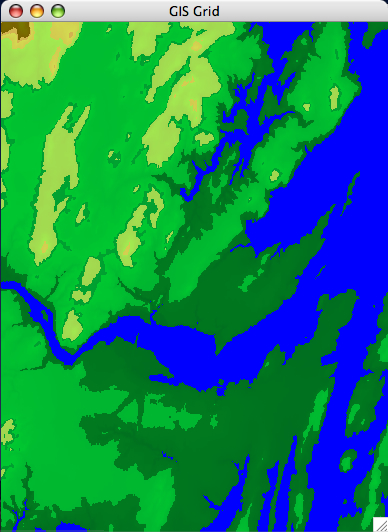
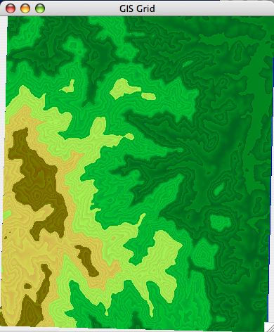
For the rendering part, I am most interested in the looks of your rendering. Play with colors, and make it look like a real map. On a real map elevations are coded using colors: high elevations are brown, low elevations are green. Here are some good ones.
|
|
|
| [Brunswick DEM] | [set1 DEM] |
Extensions
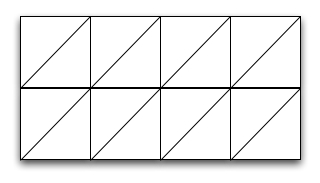
So far you render a terrain by rendering each point separately. In general rendering of a surface is of better quality if the surface is represented as a triangular mesh rather than a discrete set of points (the graphics engine can compute normals to the surface to determine lighting, reflection and all sorts of other stuff). An improved renderer would view the grid as a set of triangles (see below). Instead of drawing points, draw lines between neighboring points so that overall the lines form a triangulation as below. To decide the color of a line, consider its height to be the average height of its endpoints.
The goal of flow modeling is to quantify how much water flows through any point of the terrain. Flow reveals a lot of information about the terrain: The points with a lot of flow will be on the river network, while the points with low flow will be on the ridge network of the terrain. Knowledge about flow on the terrain turns out to be the fundamental step in many geographical processes. Unfortunately, flow data is not available from satellites, like elevation data. The location of rivers can be obtained by flying a plane and identifying rivers, but you can imagine that is a very very expensive process. That is why people have looked into ways to model flow based on the elevation of the terrain.
For a grid terrain flow is expressed by a flow grid which has the same size as the elevation grid.
Grid flowGridThe value of this flow grid at position (i,j) represents the total amount of flow that flows through point (i,j).
Imagine that initially every single point in the grid has 1 unit of water. So the very first thing that you want to do in computeFlow() after you create the flow grid is
for (int i=0; i < rows; i++)
   for (int j=0; j < cols; j++)
     if point is not NODATA then flowGrid.set(i,j, 1);
     else flowGrid.set(i,j,NODATA);
Here assume you have a setter on a Grid flowGrid.set(i,j,
val) that sets the value of an element (i,j) to the desired
value.
The question is how to model the flow of water? The simplest way to model the flow is to assume that every single point in the grid distributes its water (initial, as well as incoming) to a single neighbor, namely its steepest downslope neighbor. If there are ties, they are broken arbitrarily.
So you see, with this model water follows the steepest way down, either to the edge of the terrain or to a pit. Because water flows "down", there cannot be cycles.
The goal is to compute, for each point in the grid, the total amount of water that flows through that point.
The first method that you'll write will be:
boolean flowsInto(int i, int j, int k, int l)which returns true if cell (i,j) flows into cell (k,l), that is, if cell (k, l) is the steepest downslope neighbor of cell (i,j). The way this method works is the following: it looks at all 8 neighbors of cell (i,j) and computes the lowest neighbor; this is the direction where water would go from cell (i,j). Then it checks whether this neighbor is equal to (k,l), in which case it returns true; otherwise it returns false.
Once you have method flowsInto written and tested, you can start working on computing flow. You will write a method that computes a flow-accumulation grid based on the (elevation) grid:
Grid computeFlow() {

    // create flow grid; you will need to write this constructor
   Grid flowGRid  = new Grid (rows, cols, etc);

   //initialize flow grid
    for (int i=0; i< rows; i++) {
	for (int j=0; j < cols; j++) {
	 ...
	}
    }

    //compute flow grid
    for (int i=0; i< rows; i++) {
	for (int j=0; j < cols; j++) {

           //compute flow of point (i,j)
	   int flow = computeFlow(i, j, ...);

           flowGrid.set(i,j, flow);
	}
    }


   return flowGrid;
}
Naturally, you will write a separate method
computeFlow(i,j,...) that computes the flow of a point (i,j).
The way I envision the computation of the flow of a cell (i, j), is
that you will run a loop through all its neighbors, for every neighbor
you will check whether it flows into the current cell, and if it does,
you will add its value of the flow to the flow of the current cell.
Note that a cell can receive flow from multiple cells. Also note that
you will need to compute the value of the flow of the neighbor, which
means that the problem is probably recursive.
The basic thing to note is when recursion stops. When no neighbor flows into the current cell there are no subsequent recursive calls.
The most important thing to think about is how to avoid computing the flow of a cell multiple times. One obvious way is to mark the grid: initially the entire grid is unmarked; whenever you determine the final value of the flow of cell (i,j), you set mark[i][j] = true. This way you know, if you ever need flow[i][j], whether you've computed it before or not. Marking the grid is just one way to do it ---it may make things clearer, or not. Maybe marking is not necessary at all in this case; if you think you can do without marking the grid, do so.
For debugging reasons, you should first get test2.asc to compute flow correctly. Some test files are here. Here is how the grid test2.asc looks like:
The grid is:
 9 9 9 9 9
 8 7 6 7 8
 7 6 5 6 7
 6 5 4 5 6
 5 4 3 4 5
Here is what the flow should look like:
The grid is:
 1 1 1 1 1
 1 2 4 2 1
 1 2 9 2 1
 1 2 14 2 1
 1 3 25 3 1
Note that point (4, 2) has height 3, and receives flow from all its neighbors, as it is the lowest neighbor for each of them. So 2 + 3 + 14 + 2 + 3 = 24. Add to this the initial 1 unit of flow at point (4, 2) and you got 25.
If you got test2.asc to run correctly, then your program is almost correct except maybe nodata values.
This will work, but will not look that good. Basically, you need a diferent color map for flow than you need for elevation. For a perfect lab, you would write a new render method especially for a flow grid. Why? On a flow grid the intervals/buckets for colors need to be much more aggressive, because there are very few cells with high values of flow. If you spread the range of heights uniformly over the color range, the rivers will not show up (or maybe everything will show up blue). The idea is the same as for elevation grids, just the color details a bit different.
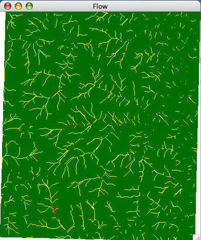
Here is how the flow of set1.asc (could) look when rendered.
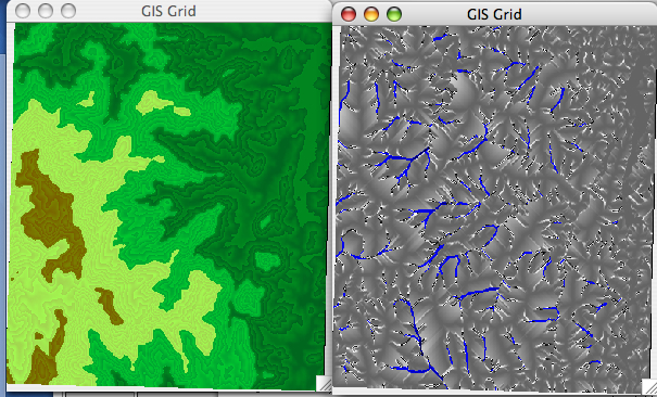
Here is another rendering of the resulting flow (different color map):
A more elegant way to do this, which I invite you to explore, is to use inheritance. Think of class Grid as handling a generic grid. You'd have Elevation Grid and a FlowGrid subclasses inheriting from Grid, both of them defining their specialized render methods.
Grid elev = new Grid("set1.asc");
elev.render();
//or, flow.renderElev() if you have a specialized method that renders elevation

Grid flow =  elev.computeFlow();
flow.render();
//or, flow.renderFlow() if you have a specialized method that renders flow
It is up to you how you deal with the different rendering methods for
an elevation grid vs a flow grid. One idea is to keep a mode
variable inside class Grid. Another idea is to simply provide two
separate functions for renderinga grid, one for rendering elevations
and one for rendering flow, and call each one when appropriate.